18.17 Correlation
Definition of Correlation
- Correlation is a statistical measure that describes the relationship between two variables.
- It can help determine if:
- Two species are associated (e.g., commonly found together).
- A species’ distribution is influenced by an abiotic factor (e.g., light, temperature, soil moisture).
Types of Correlation
- Positive Linear Correlation:
- As one variable increases, the other also increases.
- Shown by points trending upward in a scatter plot.
- Correlation coefficient (( r )) close to +1 indicates strong positive correlation.
- Negative Linear Correlation:
- As one variable increases, the other decreases.
- Shown by points trending downward in a scatter plot.
- Correlation coefficient (( r )) close to -1 indicates strong negative correlation.
- No Correlation:
- No apparent relationship between the two variables.
- Scatter plot points do not follow a trend.
- Correlation coefficient (( r )) around 0 indicates no correlation.
Correlation Coefficient (( r ))
- A value from -1 to +1 that represents the strength and direction of a correlation.
- ( r = 1 ): Perfect positive correlation.
- ( r = -1 ): Perfect negative correlation.
- ( r = 0 ): No correlation.
Methods to Calculate Correlation Coefficients
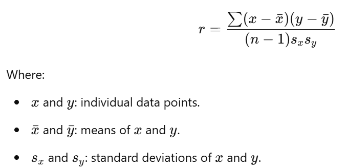
- Pearson’s Linear Correlation Coefficient:
- Used when both variables are continuous and normally distributed.
- Measures linear relationship.
- Applicable when data points appear to align along a straight line on a scatter plot.
- Spearman’s Rank Correlation Coefficient:
- Used when data is not normally distributed or if variables are ranked (ordinal data).
- Can be used for non-linear relationships.
- Suitable for data with abundance scales or ordinal rankings.
Steps for Calculating Correlation
- Draw a Scatter Plot:
- Plot data points to visually assess the relationship between the two variables.
- Look for an upward, downward, or no trend to decide if a correlation exists.
- Calculate the Correlation Coefficient:
- Use Pearson’s ( r ) for continuous, normally distributed data.
- Use Spearman’s ( rs ) for ordinal data or when distribution is uncertain.
- Interpret the Result:
- A coefficient close to +1 or -1 indicates a strong correlation.
- A coefficient near 0 indicates little or no correlation.
Worked Example: Spearman’s Rank Correlation
Scenario
An ecologist studied two plant species, common heather (Calluna vulgaris) and bilberry (Vaccinium myrtillus), on a moorland to investigate if they tend to grow together. The percentage cover of each species was recorded in 11 quadrats.
Data Collected:
| Quadrat | % Cover of C. vulgaris | % Cover of V. myrtillus |
|---|---|---|
| 1 | 30 | 15 |
| 2 | 37 | 23 |
| 3 | 15 | 6 |
| 4 | 15 | 10 |
| 5 | 20 | 11 |
| 6 | 9 | 10 |
| 7 | 3 | 3 |
| 8 | 5 | 1 |
| 9 | 10 | 5 |
| 10 | 25 | 17 |
| 11 | 35 | 30 |
Steps to Calculate Spearman’s Rank Correlation (( rs )):
- Formulate a Hypothesis:
- Null Hypothesis (H₀): There is no correlation between the percentage cover of C. vulgaris and V. myrtillus.
- Rank the Data:
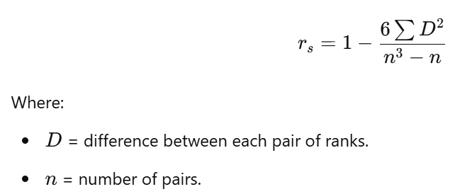
- Rank each set of data points separately for C. vulgaris and V. myrtillus.
- Calculate the difference (( D )) between ranks for each quadrat.
- Calculate ( rs ) Using Spearman’s Formula:
- Interpret the Result:
- The ecologist calculated ( rs = +0.930 ), indicating a strong positive correlation.
- The null hypothesis is rejected in favor of the alternative hypothesis that there is a correlation between the two species.
Conclusion:
- There is a strong positive correlation between the abundance of C. vulgaris and V. myrtillus, suggesting they tend to grow together.
Worked Example: Pearson’s Linear Correlation
Scenario
A student studied pine trees to investigate if larger trees (measured by circumference) have wider cracks in their bark.
Data Collected:
| Tree Number | Circumference (m) | Mean Crack Width (mm) |
|---|---|---|
| 1 | 1.77 | 50 |
| 2 | 1.65 | 28 |
| 3 | 1.81 | 60 |
| 4 | 0.89 | 24 |
| 5 | 1.97 | 95 |
| 6 | 2.15 | 51 |
| 7 | 0.18 | 2 |
| 8 | 0.46 | 15 |
| 9 | 2.11 | 69 |
| 10 | 2.00 | 64 |
| 11 | 2.42 | 74 |
| 12 | 1.89 | 69 |
Steps to Calculate Pearson’s Correlation (( r )):
- Formulate a Hypothesis:
- Null Hypothesis (H₀): There is no correlation between tree circumference and crack width.
- Draw a Scatter Plot:
- Plot tree circumference on the x-axis and crack width on the y-axis.
- The scatter plot shows an upward trend, suggesting a potential positive correlation.
- Calculate Pearson’s ( r ) Using the Formula:
- Interpret the Result:
- The student calculated ( r = 0.79 ), indicating a moderate to strong positive correlation.
- The null hypothesis is rejected.
Conclusion:
- There is a positive correlation between tree circumference and crack width, suggesting that larger trees tend to have wider cracks.
Key Terms
- Pearson’s Linear Correlation: Measures linear correlation between two normally distributed variables.
- Spearman’s Rank Correlation: Measures correlation for ranked or non-linear data, or when normal distribution cannot be confirmed.
- Correlation Coefficient (( r )): Indicates strength and direction of a correlation.
Summary
- Correlation helps to identify relationships between variables, such as species associations or the effect of abiotic factors on species distribution.
- Spearman’s rank is used for ordinal or non-linear data, while Pearson’s linear is used for normally distributed, continuous data.
- Both correlation methods provide insights but do not imply causation.