17.06 Hardy–Weinberg Principle
Hardy–Weinberg Principle:
- The Hardy–Weinberg Principle is a foundational concept in population genetics that allows the calculation of allele and genotype frequencies within a large, randomly mating population. This principle provides a null model against which evolutionary changes can be measured, assuming that certain conditions are met to prevent evolution.
1. Introduction to the Hardy–Weinberg Principle
- The Hardy–Weinberg Principle, formulated independently by G.H. Hardy and Wilhelm Weinberg in 1908, serves as a mathematical framework to study genetic variation in populations. It posits that allele and genotype frequencies will remain constant from generation to generation in the absence of evolutionary influences. This equilibrium state is known as Hardy–Weinberg Equilibrium (HWE).
Importance:
- Baseline for Evolutionary Studies: It allows scientists to determine whether or not evolution is occurring in a population by comparing observed genetic data with expected frequencies under HWE.
- Predictive Tool: Facilitates predictions about genetic variation over generations.
2. Key Components of the Hardy–Weinberg Principle
- To apply the Hardy–Weinberg Principle, several key components and assumptions must be understood:
2.1 Allele Frequencies in a Population
Consider a gene with two alleles:
- A (dominant allele)
- a (recessive allele)
Let:
- p = frequency of the dominant allele A
- q = frequency of the recessive allele a
Since there are only two alleles: p+q=1(Equation 1)
Calculation of Allele Frequencies: If the frequency of one allele is known, the frequency of the other can be easily determined using Equation 1.
2.2 Genotype Frequencies
There are three possible genotypes in a population with two alleles:
- AA (homozygous dominant)
- Aa (heterozygous)
- aa (homozygous recessive)
The Hardy–Weinberg Principle provides equations to calculate the expected genotype frequencies:
- AA (homozygous dominant): p2
- Aa (heterozygous): 2pq
- aa (homozygous recessive): q2
Thus, the sum of all genotype frequencies is:
p2 +2pq+q2 =1(Equation 2)
Understanding Genotype Frequencies:
- p2: Represents the proportion of individuals with two dominant alleles.
- 2pq: Represents the proportion of heterozygous individuals.
- q2: Represents the proportion of individuals with two recessive alleles.
3. Mathematical Foundation of the Hardy–Weinberg Principle
The principle is derived from the binomial expansion of (p+q)2(p + q)^2(p+q)2, which represents the possible combinations of alleles during gamete formation.

This expansion corresponds to the genotype frequencies:
- p2: AA
- 2pq: Aa
- q2: aa
This mathematical relationship underpins the predictions of genotype frequencies under HWE.
4. Assumptions of the Hardy–Weinberg Principle
For a population to be in Hardy–Weinberg Equilibrium, the following conditions must be met:
- Large Population Size (No Genetic Drift):
- Reason: Prevents random fluctuations in allele frequencies.
- Implication: Small populations are more susceptible to changes in allele frequencies due to chance.
- No Mutation:
- Reason: Ensures allele frequencies remain unchanged by new mutations introducing new alleles or altering existing ones.
- No Migration (No Gene Flow):
- Reason: Prevents the introduction or removal of alleles from the population through the movement of individuals.
- Random Mating:
- Reason: Ensures that individuals pair by chance, not based on genotype or phenotype, maintaining existing allele frequencies.
- No Selection (No Natural Selection):
- Reason: Prevents certain alleles from being favored or disfavored, ensuring allele frequencies remain constant.
Impact of Violating Assumptions:
- Genetic Drift: Can cause allele frequencies to fluctuate randomly, especially in small populations.
- Mutation: Introduces new alleles or changes existing allele frequencies.
- Migration: Alters allele frequencies by adding or removing alleles.
- Non-Random Mating: Can change genotype frequencies without altering allele frequencies.
- Selection: Alters allele frequencies based on differential survival and reproduction.
5. Applications of the Hardy–Weinberg Principle
Understanding HWE allows biologists to:
5.1 Test for Evolutionary Forces
- By comparing observed genotype frequencies with those predicted by HWE, scientists can infer whether evolutionary forces are acting on a population.
- No Significant Difference: Suggests the population is in HWE, and no evolution is occurring.
- Significant Difference: Indicates that one or more of the HWE conditions are not met, implying that evolutionary forces (e.g., selection, genetic drift, gene flow) may be at play.
5.2 Estimate Carrier Frequencies
HWE can estimate the frequency of carriers (heterozygotes) for recessive genetic disorders.
- Example: In a population where 1% exhibit a recessive disorder (aa), HWE can estimate the carrier frequency (Aa).
5.3 Conservation Biology
Helps in managing genetic diversity in endangered species by monitoring allele frequencies.
6. Statistical Testing: The Chi-Squared (χ²) Test
- The Chi-Squared test assesses whether the observed genotype frequencies significantly deviate from those expected under HWE.
Steps in Chi-Squared Test:
- Calculate Expected Genotype Frequencies:
- Use HWE equations (p2, 2pq, q2) based on allele frequencies.
- Determine Observed Genotype Frequencies:
- Obtain from empirical data or experiments.
- Apply the Chi-Squared Formula:

- Oi = Observed frequency of genotype iii
- Ei = Expected frequency of genotype iii
- Determine Degrees of Freedom: Degrees of Freedom = 3 − 2 = 1
- Compare χ² Value to Critical Value:
- Using a χ² distribution table and the determined degrees of freedom, ascertain whether to reject the null hypothesis (that the population is in HWE).
Interpreting Results:
- χ² < Critical Value: Fail to reject the null hypothesis; population is in HWE.
- χ² ≥ Critical Value: Reject the null hypothesis; population is not in HWE.
7. Worked Example Questions
Example Problem 1:
- Problem: If 16% of a population exhibits the homozygous recessive genotype dd, calculate the proportions of DD (homozygous dominant) and Dd (heterozygous) individuals.
Solution:
- Identify Given Information:
- Frequency of homozygous recessive genotype (dd): 16% or 0.16
- Let d represent the recessive allele.
- Therefore, q2=0.16
- Calculate Allele Frequencies:

- Calculate Genotype Frequencies:

- Verification:
- Sum of genotype frequencies:
0.36+0.48+0.16=1 (or 100%)
- Sum of genotype frequencies:
Answer:
- DD: 36%
- Dd: 48%
Example Problem 2:
- Problem: In a population of 10,000 individuals, 1,000 exhibit the recessive phenotype tt. Assuming the population is in Hardy–Weinberg Equilibrium, calculate the allele frequencies T and t, and determine the number of heterozygous individuals Tt.
Solution:
- Identify Given Information:
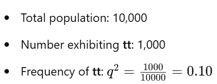
- Calculate Allele Frequencies:

- Calculate Genotype Frequencies:

- Verification:
- Total individuals: 4,672 + 4,328 + 1,000 = 10,000
Answer:
- Allele Frequencies:
- T (p): ≈ 0.6838
- t (q): ≈ 0.3162
- Number of Heterozygous (Tt) Individuals: 4,328
8. Extended Applications and Considerations
8.1 Multiple Alleles and Multiple Genotypes
- While the basic Hardy–Weinberg model considers two alleles, many genes have multiple alleles. The principle can be extended to accommodate multiple alleles using similar principles but requires more complex calculations.
Example: ABO Blood Group System
- Alleles: IA, IB, i
- Genotypes: IAIA, IAIB, IAi, IBIB, IBi, ii
- Frequency Calculations: Extend the principle to account for the third allele.
8.2 Partial Dominance and Incomplete Dominance
- The Hardy–Weinberg equations assume complete dominance. However, in cases of incomplete dominance or co-dominance, phenotype frequencies may not align directly with genotype frequencies, necessitating adjustments in calculations.
Example: Snapdragon Flower Color
- Alleles: R (red), r (white)
- Heterozygote (Rr): Pink
- Phenotype Ratios: Different from the standard dominant-recessive model.
8.3 Polygenic Traits
- For traits controlled by multiple genes (polygenic), Hardy–Weinberg calculations become more complex, as multiple loci contribute to the overall phenotype. While the principle still applies, allele frequency calculations must consider each gene separately.
9. Limitations of the Hardy–Weinberg Principle
- While the Hardy–Weinberg Principle is a powerful tool, it has limitations:
- Simplistic Assumptions: Real populations often violate HWE assumptions, making exact equilibrium rare.
- Detection Sensitivity: Small deviations from HWE can be difficult to detect without large sample sizes.
- Not Predictive for Evolution: It does not predict allele frequencies over time under evolutionary pressures; instead, it provides a snapshot under equilibrium.
- Ignores Epistasis and Linkage: Interactions between genes and linked genes are not accounted for, which can influence genotype frequencies.
Real-World Considerations:
- Population Structure: Subpopulations with different allele frequencies can affect overall HWE calculations.
- Selection Pressures: Environmental factors can favor certain alleles, disrupting equilibrium.
- Cultural Practices: Non-random mating practices (e.g., assortative mating) can influence genotype frequencies.
10. Additional Practice Problems
- Problem 3: In a certain population, 64% of individuals are homozygous dominant (CC). Assuming the population is in Hardy–Weinberg Equilibrium, calculate: a) The frequency of the recessive allele (c). b) The expected frequency of heterozygous (Cc) individuals. c) The number of Cc individuals in a population of 2,500.
Solution:
a) Calculate Allele Frequencies:

b) Calculate Heterozygous Frequency:
- 2pq = 2 × 0.8 × 0.2 = 0.322
Answer b: Expected frequency of Cc = 0.32 or 32%
c) Calculate Number of Heterozygotes:
- Total population = 2,500
- Number of Cc individuals = 0.32 × 2500 = 8000.
Answer c: 800 Cc individuals
Problem 4: In a population of birds, the allele for blue feathers (B) is dominant over the allele for green feathers (b). If 9% of the population exhibits green feathers, assume the population is in Hardy–Weinberg Equilibrium and determine: a) The allele frequencies of B and b. b) The percentage of heterozygous (Bb) birds. c) The number of heterozygous birds in a population of 5,000.
Solution:
a) Calculate Allele Frequencies:

Answer a: Frequency of B (p) = 0.7; Frequency of b (q) = 0.3
b) Calculate Heterozygous Frequency:
- 2pq = 2 × 0.7 × 0.3 = 0.42 or 42%
Answer b: 42% heterozygous (Bb) birds
c) Calculate Number of Heterozygotes:
- Total population = 5,000
- Number of Bb birds = 0.42 × 5000 = 2,100
Answer c: 2,100 heterozygous birds
Worked Example Questions
Example Problem:
- If 16% of a population exhibits the homozygous recessive genotype dd, calculate the proportions of DD (homozygous dominant) and Dd (heterozygous) individuals.
Solution:
